One of my lab mates wanted to calculate bootstrap CIs for a project, which is something I know how to do. So I wanted to write a basic tutorial on bootstrap confidence intervals.
Author
Zane Billings
Published
October 9, 2023
In this blog post, I’m going to go over a short example of using the nonparametric bootstrap to construct confidence intervals for arbitrary statistics. Exact and asymptotic limits are all great, but unfortunately they have to exist before you can calculate them, and these methods are often very analytically difficult (requiring, e.g., Taylor series analysis). We can often trade off computational power for analytical problem solving using the bootstrap method to construct pretty good confidence intervals instead.
I’ll start by going over what I think is the most intuitive approach for bootstrap CIs, the percentile method. This method has some limitations though, so I’ll talk about the BCa adjustment which can produce better results, and I’ll talk about how to get these CIs with the boot package in R.
Example problem setup
For an example, we’ll make some simulated data that’s similar to the situation where we actually need to use a bootstrap CI in my lab group’s research. We’ll consider a fairly simple example: in a study sample of size \(n = n_t + n_p\), where \(n_t\) people get a vaccine and \(n_p\) people get a placebo. They are followed up for an appropriate amount of time (or challenge with virus, your choice), and we record which individuals get infected and which do not. For this simulated example, the effect we are interested in measuring is the vaccine effectiveness, which can be calculated from the risk ratio. That is, \[\mathrm{VE} = 1 - \mathrm{RR} = 1 - \frac{\text{risk in vaccine group}}{\text{risk in placebo group}}.\] To do this, we’ll simulate infection data for both groups. If we want our target VE to be, say, \(75\%\), we want the risk ratio to be \(25\%\), and we can set the two prevalences however we want, as long as they are sensible prevalences (between \(0\%\) and \(100\%\)) and their ratio is \(\frac{1}{4}\). So for ease of computation, let’s say that the risk in the vaccine group is \(10\%\) and the risk in the placebo group is \(40\%\). Let’s simulate 100 patients where 50 are in the placebo group and 50 are in the vaccine group.
set.seed(134122)n <-100Lsim_dat <- tibble::tibble(# Treatment is 0 for placebo, 1 for vaccinatedtreatment =rep(c(0, 1), each = n /2),outcome =rbinom(n, size =1, prob =rep(c(0.4, 0.1), each = n /2)))table( sim_dat$treatment, sim_dat$outcome,dnn =c("treatment", "outcome")) |>addmargins()
         outcome
treatment   0   1 Sum
      0    27  23  50
      1    43   7  50
      Sum  70  30 100
If we look at our table, we see that we get estimated risks of \(23/50 = 46\%\) in the placebo group, and \(7/50 = 14\%\) in the vaccine group, giving us an observed VE of \(1 - 0.3043 \approx 70\%.\) This is close to what we know is the true VE in the simulation, but different enough that we can immediately see the effect of sampling variability. Of course, as we simulate increasingly more people, we will get a more accurate estimate of the VE.
Now, we might want to construct a confidence interval for our sample, which would ideally cover the true VE. But we forgot all the different methods for building confidence intervals for the risk ratio, no matter how many of them they taught us or how many times we covered it during epidemiology class. (Or if you’re like me, you did an epidemiology PhD without any intro to epi classes and never really learned…) So fortunately for us, nonparametric bootstrapping provides a really convenient and flexible way to “automatically” get a CI, as long as we have a relatively modern computer – even though bootstrapping is called a computer intensive method, for simple statistics like this one, you can get bootstrap intervals pretty fast even on cheap hardware.
Constructing resamples
The first step of computing a bootstrap CI is to construct the bootstrap distribution. Bootstrapping refers to a specific type of resampling process that’s similar to cross-validation or leave-one-out methods. Call our entire data set \(D\). We construct a bootstrap resample \(D_i\) (\(i = 1, 2, \ldots, B\) where \(B\) is the number of bootstrap resamples we do) by sampling with replacement\(n\) records from \(D\). This means that each resample can have the same observation repeated multiple times, and does not have to include every observation (in fact, we can use the bootstrap similarly to cross-validation for model tuning by using the bootstrap resample as the analysis set and the points not included in the resample as the assessment set). We resample in this way specifically, because it leads to specific properties (under certain regularity conditions) which allow our confidence intervals to work correctly. (Math details omitted since they’re complicated and honestly not too important for what we’re trying to do here.)
We could of course do this by hand.
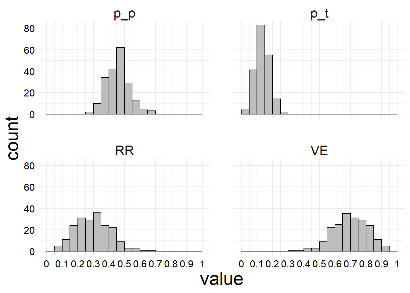
set.seed(3547512)B <-199Lres <-matrix(nrow = B, ncol =4)colnames(res) <-c("p_p", "p_t", "RR", "VE")for (i in1:B) {# Sample the data indices that we should use for this sample idx <-sample.int(nrow(sim_dat), replace =TRUE) D_i <- sim_dat[idx, ]# Code to calculate the risk in the placebo group and the risk in the# treatment group# We could write this in a much more compact/efficient way, but I did it# this way for readability p_p <- D_i |> dplyr::filter(treatment ==0) |> dplyr::pull(outcome) |>mean() p_t <- D_i |> dplyr::filter(treatment ==1) |> dplyr::pull(outcome) |>mean() RR <- p_t / p_p# Store results in output matrix res[i, 1] <- p_p res[i, 2] <- p_t res[i, 3] <- RR res[i, 4] <-1- RR}res <- tibble::as_tibble(res)print(res, n =6)
This gives us a resampling or bootstrap distribution with 199 values for each of the calculated values (\(p_p\), \(p_t\), the \(\mathrm{RR}\), and the \(\mathrm{VE}\)). We can look at those distributions. (I’ll briefly explain why we might choose 199 in a moment.)
Here we only do 199 resamples because the program I wrote is super inefficient and doing much more would take a while. (Although it is worthwhile to note that the calculation of bootstrap statistics is trivially parallelizable, so with access to sufficient resources, even a computationally expensive or poorly implemented statistic can be computed in a reasonable amount of time.)
So now that we have calculated a bootstrap distribution for our statistic of interest (the VE, along with its component statistics as recordkeeping), how do we estimate the CI from this distribution? In my opinion, the most intuitive way is to use the percentile method.
Percentile method
Before introducing the percentile method, we should note that many people on the internet will complain and moan about how “bad” this method is, including Davison and Hinkley (who did it in their book that is older than stack exchange or whatever). People like to moan about how it is not quite right, but as Efron (bootstrap inventor and expert) and Hastie put it, the goal of bootstraps is to have wide applicability and close to perfect coverage. So this method is, in general, pretty good in a wide variety of cases. Especially if we think about all the errors that get compounded in the process of observing and analyzing real-world data, something as trivial as being a few coverage percentage points off from \(95\%\) is really not something to cry about, especially when we can construct intervals for arbitrarily complicated statistics. So, let’s define the method.
The percentile method indeed is so simple that skepticism is natural. Whereas other bootstrap methods rely on finding normalization transformations to ensure correct confidence limits, the percentile method relies only on the existence of such a transformation, which can be unknown to us, as this method is scale-invariant. This method literally just involves calculating the closest empirical quantiles of interest to those we are interested in. Using the percentile method, a \(95\%\) confidence interval for the VE would be \[\left( \mathrm{VE}^{*}_{(B+1)(0.025)}, \mathrm{VE}^{*}_{(B+1)(0.975)} \right)\]
So if we chose \(B=199\), then we would order our observed statistics, and our percentile method CI would be formed by the 5th entry in that vector and the 195th entry in that vector. For such ease of computation, \(B = 399\) or \(599\) and so on are often used to ensure the quantiles are exact. However, again, this is an example of sweating over tiny amounts of CI coverage that likely are not too important to begin with, so choosing a nice round number like \(B = 2000\) is often sufficient. Typically, you need at least \(B = 1000\), though \(B = 10000\) (or \(9999\ldots\)) is even better and typically not even too computationally demanding on modern machines. So, for our example, our percentile CI for the VE would be calculated as follows.
sort(res$VE)[c(5, 195)]
[1] 0.4441367 0.9032258
R has a lot of quantile algorithms, but we can specifically use Type 1 or 2 to get the same estimates (2 is probably better if you don’t use a \(B\) ending in 9’s). The others are all fairly similar though and like I said, I really don’t think being upset about the amount of difference you get between quantile algorithms really matters.
quantile(res$VE, probs =c(0.025, 0.975), type =1)
     2.5%     97.5%
0.4441367 0.9032258
So, we would pair this with our empirical estimate of the VE (we could take, e.g. the mean of the bootstraps, which should always be similar to the overall estimate we already got) to get an estimated VE of \[\widehat{VE} = 69.57\% \
\left(95\% \text{ CI: } 44.41\% \ - \ 90.32\%\right).\] Now that is maybe not the most precise estimate of VE in the world, but based on the bootstrap percentile method, it at least seems that our vaccine is conferring some protection, with the possibility of a pretty good amount. And the CI covers our true estimate, as we would hope (although it’s important to remember that we could’ve gotten unlucky with the random sample we drew, and if our CI didn’t cover the true estimate on one experiment, that doesn’t mean the CI is flawed). Note that we would expect this CI to get smaller as \(n\) increases, but not as \(B\) increases. Increasing \(B\) decreases the “Monte Carlo” (MC) error, or random error introduced by the random process involved in the algorithm, but doesn’t do anything about the actual sampling error.
Of course, like I said, some people really don’t like the percentile method. So we can instead appeal to a much more complicated method devised by Efron and some coworkers called the BCa method, and I’ll show how to automate the calculation of these CIs.
BCa method and boot
The bias-corrected and accelerated (BCa) percentile method introduces, as you might guess, new complications to reduce the bias and accelerate the convergence of the percentile bootstrap method. Davison and Hinkley agree with Efron and Hastie that this method fixes many of the issues with the basic percentile CI, and there are not really any major objections in the same way that there are for the percentile method. However, this method can be more computationally intensive and certainly more demanding to calculate, and as such I do not recommend implementing in by hand in everyday situations. The central problem here is the estimation of the acceleration parameter \(a\), although there is fortunately a nonparametric estimator that works well in many situations.
So, we will use the boot package.
library(boot)
The first step to getting bootstrap CIs via boot is to write a function with a specific order of arguments. The first argument passed to this function will be the original data, and the second will be a vector of indices which are sampled by the bootstrapping procedure. Additional arguments are allowed. For our problem, a function might look like this.
est_VE <-function(data, idx) {# Sample the data indices that we should use for this sample D_i <- data[idx, ]# Code to calculate the risk in the placebo group and the risk in the# treatment group p_p <-mean(subset(D_i, treatment ==0)$outcome) p_t <-mean(subset(D_i, treatment ==1)$outcome) RR <- p_t / p_p# Return the VEreturn(1- RR)}
Next, we need to create a resampling object using the boot::boot() function. I’ll comment the important arguments in the code chunk. There are many other arguments we could pass in, and the details of those are described in the manual or in Davison and Hinkley (see references). In particular, the parallel, cl, and ncpus arguments can be used for easy parallel computing.
set.seed(7071234)VE_boot <- boot::boot(# First argument is the data framedata = sim_dat,# Second argument is the function we want to calculate on resamplesstatistic = est_VE,# R is the number of resamples, which I called B beforeR =9999,# We want to use ordinary nonparametric bootstrap -- this is the default# but I wanted to emphasize itsim ="ordinary")
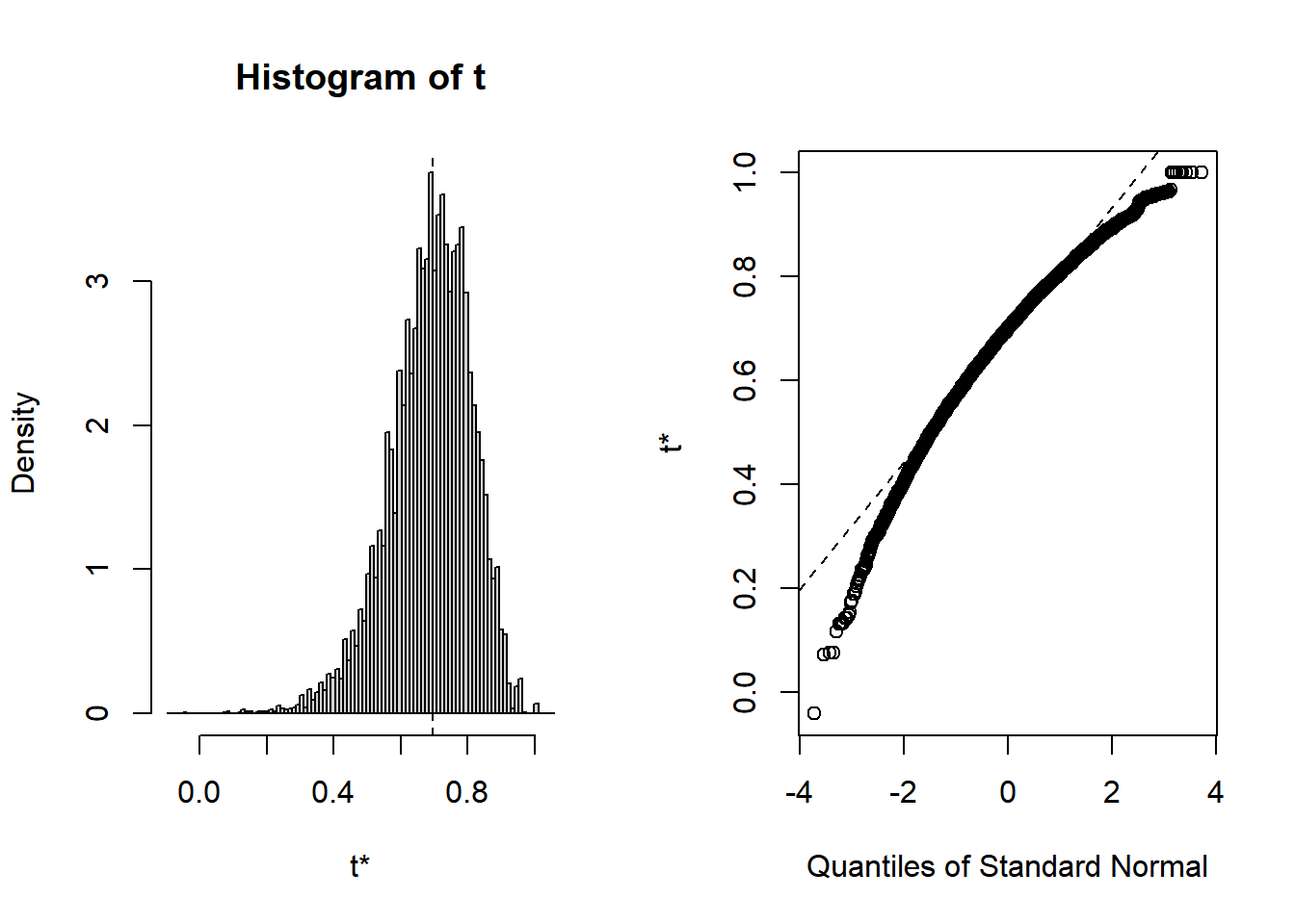
Because the boot package is optimized so well, that seems like it actually took less time than my simple example earlier. If we just print the object, we can see the estimated statistic and bootstrap SE.
We can see that it is nonnormal, with a long left tail. Such nonnormality indicates that the normal approximate bootstrap method (which I didn’t discuss) is not appropriate, and the BCa method is generally much better in this case.
There is a lot you can do with this package that I am not going to talk about and don’t really know about. But the next thing we want to do for this example is compute those BCa confidence intervals. Fortunately for us, we can actually calculate all the types of CI available with one function call. Note that we could also compute the “studentized” CI, but that requires us to specify variances for each observation.
BOOTSTRAP CONFIDENCE INTERVAL CALCULATIONS
Based on 9999 bootstrap replicates

CALL :
boot::boot.ci(boot.out = VE_boot, conf = 0.95, type = c("norm",
    "basic", "perc", "bca"))

Intervals :
Level      Normal              Basic
95%   ( 0.4633,  0.9429 )   ( 0.4991,  0.9807 )

Level     Percentile            BCa
95%   ( 0.4106,  0.8922 )   ( 0.3701,  0.8778 )
Calculations and Intervals on Original Scale
We can see that the percentile CI is quite similar to the one we got by hand, which is nice and the difference is likely attributable to random error. Notice, however, that the normal and basic intervals are shifted upwards from the percentile interval, and the BCa interval is shifted down. The BCa interval is corrected for bias, which is why it is shifted down (in Efron and Hastie they discuss why our CIs might be biased upwards to begin with). In this case, the different intervals are actually a bit different, although again I’m not sure how useful it is to fret over whether the lower limit of the CI for our VE is \(41\%\) or \(37\%\). (But I do admit that a range of \(46\%\) to \(37\%\) across methods is not ideal, though I don’t know that these two estimates would change any qualitative decisions that you might make based on the analysis. But either way the normal method is not great, and I don’t love the basic method, which is why I didn’t recommend using either of those.)
In general I would use the BCa limits, since they are the least controversial, technically the “best” in a specific sense, and are just as easy to calculate. And it’s important to note that all of these CIs cover our true parameter for this simulated experiment; to truly investigate the convergence and bias properties of these different CIs we would need to run many simulated experiments.
Conclusions
In this tutorial, we simulated data and got confidence intervals using two different bootstrap methods for the VE from a theoretical vaccine study. We demonstrated how easy it is to obtain BCa intervals using the boot package in R.
We should note that bootstrapping does not solve any issues induced by having too low of a sample size – bootstrap CIs will often be just as bad as any other CIs if the sample size is quite small. If I were to keep writing this blog post, I would compute several of the other alternative CIs for the VE, like the normal approximate and whatever exact CIs people are using for that right now, I just couldn’t think of those off the top of my head and I don’t think comparing to only the normal approximate CI is useful.
There are some limitations to bootstrap, especially when we start using complex hierarchical models. But for simple CI calculations, nonparametric BCa bootstraps can often provide a decent CI estimate without requiring any analytical derivations.
References
Davison AC and Hinkley DV. Bootstrap Methods and their Applications, 1997. Cambridge University Press, Cambridge. ISBN 0-521-57391-2.
Efron B and Hastie T. Computer Age Statistical Inference, student edition, 2021. Cambridge University Press, Cambridge.
Rousselet GA, Pernet CR, Wilcox RR. The Percentile Bootstrap: A Primer With Step-by-Step Instructions in R. Advances in Methods and Practices in Psychological Science. 2021;4(1). doi:10.1177/2515245920911881.
Canty A and Ripley B (2022). boot: Bootstrap R (S-Plus) Functions. R package version 1.3-28.1.